Step 3. Combined sequence-based analysis

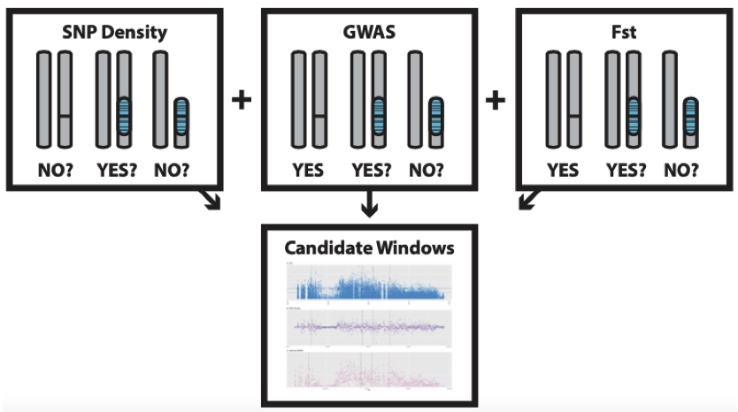
If your species of interest has a genetic basis for sex determination, but you have not been able to identify a consistent signal within your genomic data using Steps 1 and 2, the scripts for Step 3, Combined sequence-based analysis, should be able to help. If you have not identified a compelling candidate by the end of Step 3, I would suggest that there is not a genetic signal for sex determination in the genomic data you have analyzed, which was the case for sea lamprey (see the main manuscript).

In Step 3, non-overlapping signals from the reference-based methods are converted to 10kb windows and combined to increase the user’s power to focus on specific genomic regions. Once candidate windows are identified in Step 3, the user can return to GWAS, SNP density, and Fst results to determine if fixed or nearly-fixed differences exist between the sexes in the top candidate windows.

Once again, the example code Fugu_SexFindR.R and necessary input files are included in the GitHub repository in order to run the analysis for fugu and generate the plot in the SexFindR figure in the manuscript.

For the GWAS and Fst input data, parsing of the input data is carried out both in the R script, and through Python scripts and bash commands.

To generate gemma_window_count.txt which is required for the R script from fugu_gemma_sort_cut.txt (which is created in the R script from test_gemma_out.assoc.txt.zip), do the following on the command line:

sort -k1,1 -k2n fugu_gemma_sort_cut.txt > coordinated_sorted_gemma_cut.txt
python window_count.py coordinated_sorted_gemma_cut.txt gemma_window_count.txt 10000

This creates a window-based count of top GWAS hits (top 5%) within each 10 kb region across the genome.

Similarly, to generate Fstugu_window_count.txt from Fstugu_sort_cut.txt (created in R from biallelic_fst.weir.fst.zip),

sort -k1,1 -k2n Fstugu_sort_cut.txt > coordinated_sorted_Fstugu_cut.txt
python window_count.py coordinated_sorted_Fstugu_cut.txt Fstugu_window_count.txt 10000

This creates a window-based count of top Fst hits (top 5%) within each 10 kb region across the genome.

The SNP Denisty data is already in 10 kb windows from the SNP Density analysis (Step 2) and is able to be used without modifications outside of R.

With all these scripts and input data, you should be able to recreate this plot from the main manuscript in R.

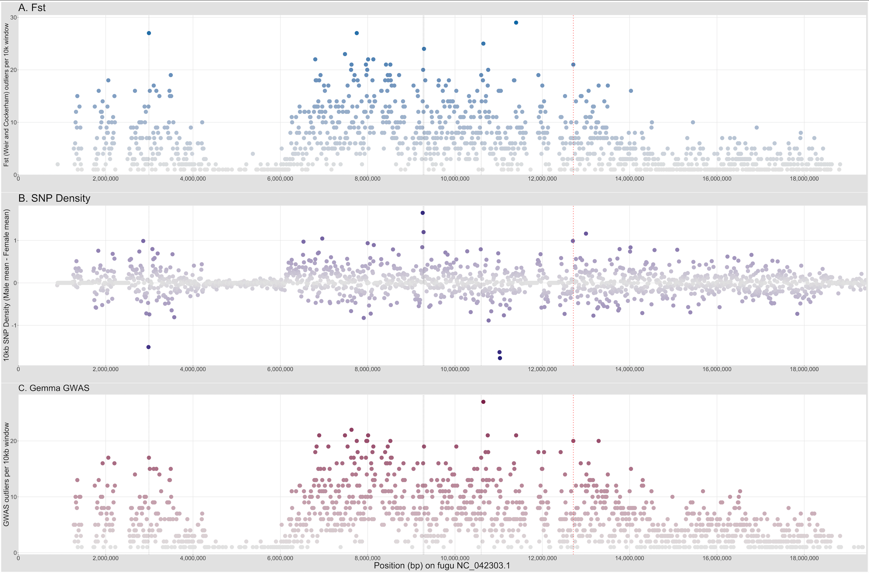
Figure 3. SexFindR Step 3 combined results identified the fugu SDR (red dotted line) alongside 4 additional candidate windows (thin black dotted lines), all on NC_042303.1. Regions of high interest are darkly colored, whereas regions of low interest are colored in grey.